In the previous post, we worked through the foundations of Bayesian inference. We saw that the posterior $p(t \mid \mathcal{D})$ is almost always intractable, and that the two main tools for approximating it are MCMC and Variational Inference. MCMC is asymptotically exact but painfully slow. VI is fast but introduces bias through its choice of approximating family. Neither scales well to the kinds of large, complex models we actually want to use in practice.
This post is about a paper that takes a completely different angle on the problem. Rather than asking “how do we approximate the posterior better?”, it asks a more radical question: what if we just directly learned to output the PPD, without ever computing the posterior at all?
That is the core idea behind Prior-Data Fitted Networks (PFNs), published at ICLR 2022. Let’s dig into how it works, why it works, and what it means for Bayesian inference more broadly.
A Quick Recap
Recall from the previous post that the quantity we actually care about for making predictions is the posterior predictive distribution (PPD):
\[p(y \mid x, \mathcal{D}) = \int p(y \mid x, t)\, p(t \mid \mathcal{D})\, dt\]This says: to predict $y$ for a new input $x$, integrate over all possible parameter values $t$, weighted by how probable each is given the data. The posterior $p(t \mid \mathcal{D})$ is just an intermediate quantity we need in order to compute this integral.
The traditional approach is to first approximate $p(t \mid \mathcal{D})$ using MCMC or VI, and then use that approximation to evaluate the integral. Both MCMC and VI pay a fresh computational cost for every new dataset you encounter. You get a new dataset, you run your sampler or your optimiser, and only then can you make predictions.
PFNs flip this on its head.
The Key Insight: Skip the Posterior Entirely
Here is the central observation: the PPD is just a function. It takes a dataset $\mathcal{D}$ and a query point $x$ as input, and it outputs a distribution over $y$. There is nothing that says you have to compute this function by first computing the posterior. You just need some way to evaluate it.
So what if you trained a neural network to approximate this function directly? You would give it a dataset and a query point, and it would output a predicted distribution over $y$, having learned to mimic what Bayesian inference would give you.
That is exactly what a PFN is. The model $q_\theta$ takes the training set $\mathcal{D}$ and a test input $x$ as input, and directly outputs an approximation to $p(y \mid x, \mathcal{D})$:
\[q_\theta(y \mid x, \mathcal{D}) \approx p(y \mid x, \mathcal{D})\]Once this model is trained, inference on a new dataset is just a single forward pass. No sampling chains, no optimisation loops. You feed in the data, you get out a distribution.
The obvious question is: how on earth do you train such a model?
The Training Objective
To train $q_\theta$, you need a loss function. The paper proposes what they call the Prior-Data Negative Log-Likelihood:
\[\ell_\theta = \mathbb{E}_{\mathcal{D} \cup \{x,y\} \sim p(\mathcal{D})}\left[- \log q_\theta(y \mid x, \mathcal{D})\right]\]Let’s unpack what this actually means, because it is surprisingly intuitive once you see it.
The key ingredient is a prior over datasets, written $p(\mathcal{D})$. This encodes your assumptions about how data is generated. For example, if you believe your data comes from a Gaussian Process with a certain kernel, then $p(\mathcal{D})$ is the distribution over datasets you would get by sampling random functions from that GP and evaluating them at random input points. If you believe your data is generated by a small neural network with random weights, then $p(\mathcal{D})$ reflects that instead.
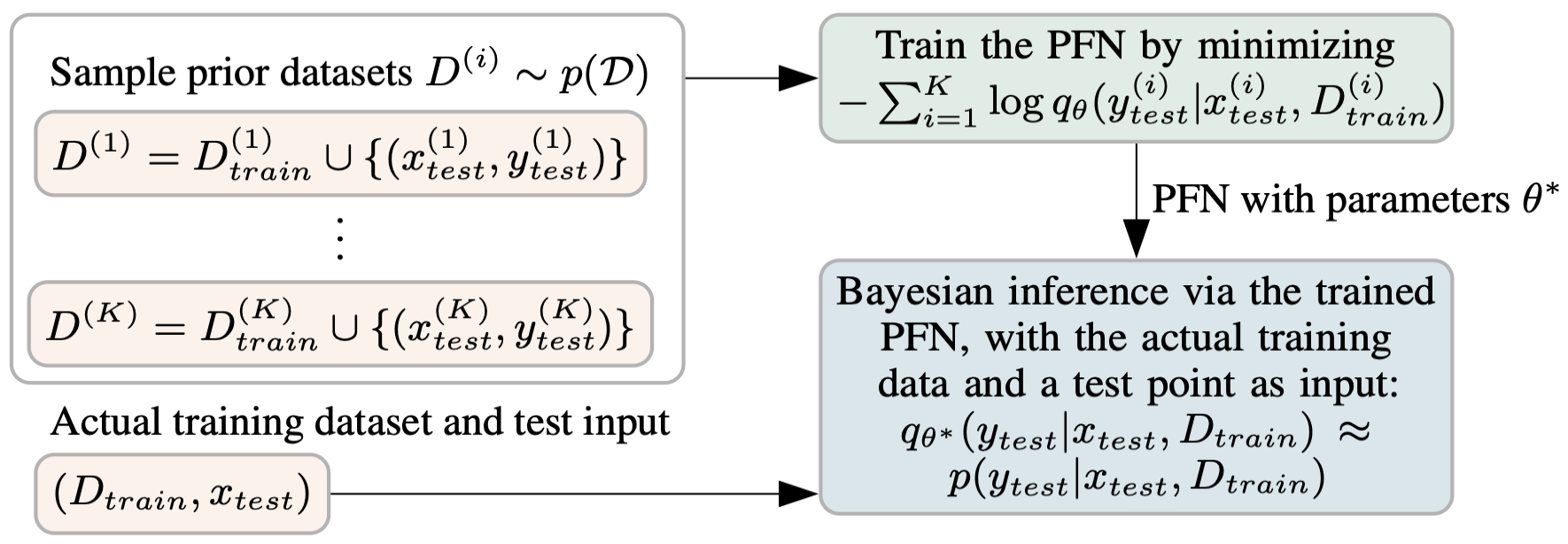
Given this prior, training works as follows. You repeatedly:
- Sample a full dataset $\mathcal{D} \cup {(x, y)}$ from the prior $p(\mathcal{D})$
- Hold out one example $(x, y)$
- Feed the remaining dataset $\mathcal{D}$ and the query point $x$ into the model
- Ask the model to predict the held-out label $y$
- Compute the negative log-likelihood of the true $y$ under the model’s predicted distribution
- Take a gradient step
This is just supervised learning. But here is what makes it special: the model is being trained across a whole distribution of tasks, not a single fixed dataset. Every training step sees a completely different dataset, drawn fresh from the prior.
Why Does This Work? The Math
It is not immediately obvious that training on synthetic datasets from a prior will teach a model to do Bayesian inference. The paper has a clean theoretical result that makes this precise. Let’s build up to it step by step.
Step 1: Rewrite the loss as an expectation over the prior.
The Prior-Data NLL is defined as an expectation over datasets sampled from the prior:
\[\ell_\theta = \mathbb{E}_{\mathcal{D} \cup \{x,y\} \sim p(\mathcal{D})}\left[- \log q_\theta(y \mid x, \mathcal{D})\right]\]We can write this expectation explicitly as an integral over all possible datasets, query inputs, and query labels:
\[\ell_\theta = -\int_{\mathcal{D},\, x,\, y} p(\mathcal{D}, x, y) \log q_\theta(y \mid x, \mathcal{D})\]Now apply the chain rule of probability: $p(\mathcal{D}, x, y) = p(\mathcal{D}, x) \cdot p(y \mid x, \mathcal{D})$. This just says that the joint probability of seeing a dataset, a query input, and a query label factorises into the probability of the dataset-input pair times the probability of the label given everything else. Substituting this in and grouping the inner integral over $y$:
\[\ell_\theta = \int_{\mathcal{D},\, x} p(\mathcal{D}, x) \left[ \int_y p(y \mid x, \mathcal{D}) \left(- \log q_\theta(y \mid x, \mathcal{D})\right) dy \right]\]The inner bracket is exactly the definition of cross-entropy between the true label distribution $p(\cdot \mid x, \mathcal{D})$ and the model’s predicted distribution $q_\theta(\cdot \mid x, \mathcal{D})$. So:
\[\ell_\theta = \mathbb{E}_{x, \mathcal{D}}\left[H\!\left(p(\cdot \mid x, \mathcal{D}),\; q_\theta(\cdot \mid x, \mathcal{D})\right)\right]\]Step 2: Connect cross-entropy to KL divergence.
Cross-entropy and KL divergence are related by a standard identity. For any two distributions $p$ and $q$:
\[H(p, q) = \text{KL}(p \,\|\, q) + H(p)\]where $H(p)$ is the entropy of $p$ alone. Plugging this in:
\[\ell_\theta = \mathbb{E}_{x, \mathcal{D}}\left[\text{KL}\!\left(p(\cdot \mid x, \mathcal{D}) \,\|\, q_\theta(\cdot \mid x, \mathcal{D})\right)\right] + \underbrace{\mathbb{E}_{x, \mathcal{D}}\left[H\!\left(p(\cdot \mid x, \mathcal{D})\right)\right]}_{\text{constant w.r.t. } \theta}\]The second term is the expected entropy of the true PPD. It does not involve $\theta$ at all, so it is just a constant from the perspective of optimisation. This means minimising $\ell_\theta$ over $\theta$ is equivalent to minimising:
\[\mathbb{E}_{x, \mathcal{D}}\left[\text{KL}\!\left(p(\cdot \mid x, \mathcal{D}) \,\|\, q_\theta(\cdot \mid x, \mathcal{D})\right)\right]\]This is the punchline. The KL divergence $\text{KL}(p | q_\theta)$ measures how different the model’s predicted distribution is from the true PPD. It is zero if and only if the two distributions are identical. So by minimising the Prior-Data NLL with standard gradient descent, you are directly pushing the model’s output toward the true PPD, averaged over all datasets that can be drawn from your prior.
Step 3: What if the model is expressive enough?
There is a nice corollary here. If the model family $q_\theta$ is rich enough to represent the true PPD exactly, then the global minimum of $\ell_\theta$ is achieved when $q_\theta(\cdot \mid x, \mathcal{D}) = p(\cdot \mid x, \mathcal{D})$ for all $x$ and $\mathcal{D}$. At that point, the KL divergence is zero everywhere. Transformers are expressive enough over set-valued inputs that this is a reasonable aspiration in practice.
The crucial practical consequence is that nowhere in this derivation did we need to compute the posterior $p(t \mid \mathcal{D})$, or evaluate the intractable normalising constant $p(\mathcal{D})$. The only thing we needed from the prior was the ability to sample datasets from it. That is a much weaker requirement than what MCMC and VI need, and it is almost always easy to satisfy.
How Training Actually Looks
Let’s make the training procedure concrete with an example. Suppose your prior is “data is generated by a Gaussian Process.”
Training proceeds like this:
- Sample a random GP function from your prior
- Evaluate it at, say, 20 random input points to get a dataset of 20 input-output pairs
- Pick one of those pairs as the held-out test point
- Feed the remaining 19 pairs plus the test input $x$ into the Transformer
- The Transformer predicts a distribution over $y$
- Compute the loss using the true $y$
- Repeat millions of times, each time with a freshly sampled GP function and freshly sampled data points
After training on millions of such synthetic datasets, the model has effectively learned what GP posteriors look like. When you then give it a real dataset at inference time and ask for a prediction, it outputs what a GP posterior would predict, in a single forward pass.
This is sometimes called meta-learning: learning at the level of tasks rather than individual examples. But PFNs are doing something more specific than generic meta-learning. Because the training distribution is grounded in a prior $p(\mathcal{D})$ that has a Bayesian interpretation, the model is not just learning to generalise across tasks. It is learning to perform Bayesian inference.
How PFNs Compare to MCMC and VI
Now that we understand how PFNs work, it is worth being precise about how they differ from MCMC and VI. The differences run deeper than just speed.
The key distinction is about when each method pays its computational cost. MCMC and VI have no offline precomputation phase. Every time you encounter a new dataset, you pay the full cost of running a sampling chain or an optimisation loop from scratch. PFNs flip this: they have an expensive offline meta-training phase, but once that is done, applying the model to any new dataset costs almost nothing.
What each method needs per new dataset:
MCMC needs to evaluate the unnormalised posterior $p(\mathcal{D} \mid t) \cdot p(t)$ at arbitrary points in parameter space. Basic methods like Metropolis-Hastings only need to query this quantity at candidate values of $t$, with no gradients required. Gradient-based variants like NUTS additionally require the likelihood to be differentiable with respect to $t$. Either way, you run a fresh sampling chain for every new dataset you encounter.
VI needs to evaluate the log likelihood $\log p(\mathcal{D} \mid t)$ and the log prior $\log p(t)$ at sampled values of $t$ in order to compute the ELBO. In practice it also needs gradients of these quantities with respect to $t$, since the ELBO is optimised via gradient descent using the reparameterisation trick. This makes differentiability a harder requirement for VI than for basic MCMC. For every new dataset, you run a fresh optimisation loop from scratch.
PFNs only need the ability to sample from the prior $p(\mathcal{D})$. This cost is paid once during offline meta-training. Once the PFN is trained, applying it to a new dataset requires no sampling, no optimisation, and no likelihood evaluations. Just a single forward pass.
A comparison:
| MCMC | VI | PFN | |
|---|---|---|---|
| Approximates | Posterior $p(t \mid \mathcal{D})$ | Posterior $p(t \mid \mathcal{D})$ | PPD directly |
| Offline precomputation | None | None | Meta-training on samples from $p(\mathcal{D})$ |
| Cost per new dataset | High (sampling chain) | Medium (optimisation loop) | Negligible (one forward pass) |
| Requires differentiable likelihood? | Only for gradient-based variants (e.g. NUTS) | Yes | No |
| Accuracy | Asymptotically exact | Biased by $q$ family | Bounded by model capacity |
The third row is the key one. MCMC and VI pay their cost fresh for every dataset. PFNs amortise the cost into meta-training and then applying them to new data is essentially free. This is the same idea behind amortised variational inference in VAEs, but applied here to the PPD directly rather than to the posterior of a single model.
Why Transformers?
You might wonder why Transformers in particular are the right architecture for this. There are a few reasons, and they are all tied to the structure of the problem.
The input is a set. A dataset $\mathcal{D} = {(x_1, y_1), \ldots, (x_n, y_n)}$ is a set of input-output pairs. Crucially, the PPD should not depend on the order in which you present those pairs. If you shuffle the training examples, your prediction for a new point should be identical. This is called permutation invariance.
Transformers handle this naturally. By removing positional encodings, the architecture becomes permutation invariant with respect to the input set. Each training pair $(x_i, y_i)$ gets encoded into a token, and the attention mechanism lets every token attend to every other token, with no sensitivity to ordering.
The input is variable-length. The number of training examples $n$ is not fixed. You might have 5 training points or 500. Transformers handle variable-length inputs natively via attention, unlike fixed-input architectures like MLPs.
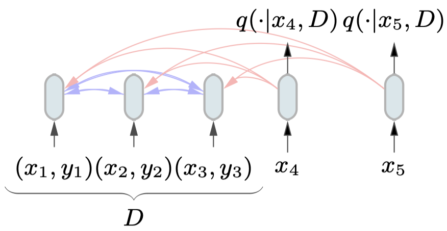
Attention mimics conditioning. In Bayesian inference, the PPD $p(y \mid x, \mathcal{D})$ involves conditioning on the entire dataset. Attention is a mechanism for dynamically routing information from one set of tokens to another. When a query point $x$ attends to all training pairs in $\mathcal{D}$, it is effectively aggregating evidence from the entire dataset to form its prediction. This is not just a metaphor; the paper shows that this actually works.
The architecture is set up so that query points can attend to all training examples, but not to each other (since predictions for different test points should be independent given $\mathcal{D}$). Training pairs attend to all other training pairs. This attention masking structure encodes exactly the right conditional independence structure for the problem.
Handling Continuous Outputs: The Riemann Distribution
One practical challenge is that the PPD for regression problems is a distribution over continuous values of $y$. Neural networks are not naturally great at this. The standard approach is to parameterise a Gaussian, but a single Gaussian is too restrictive for complex posteriors.
The paper introduces a clever solution called the Riemann Distribution. The idea is to discretise the output space into buckets and treat regression as classification over those buckets. The model outputs a probability for each bucket, and the resulting distribution is a piecewise-constant density.
The bucket boundaries are chosen so that each bucket has equal prior probability, estimated from a large sample of prior data:
\[p(y \in b) = \frac{1}{|B|} \quad \forall b \in B\]This means buckets are narrow where outputs are common under the prior, and wide where outputs are rare. The result is an adaptive discretisation that puts resolution where it matters.
For priors with unbounded support, the outermost buckets are replaced with scaled half-normal distributions to handle the tails.
The paper proves that the Riemann distribution can approximate any Riemann-integrable density to arbitrary precision by making the buckets fine enough. In practice, it works very well because neural networks are already excellent at classification, so reframing regression as classification plays to the model’s strengths.
Does It Actually Work?
The experiments in the paper are organised around three settings, going from easy to hard.
Gaussian Processes with Fixed Hyperparameters
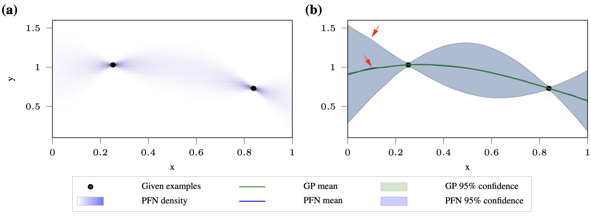
This is the sanity check. When the GP hyperparameters are fixed, the PPD has a closed form, so you can directly compare the PFN’s output to the ground truth.
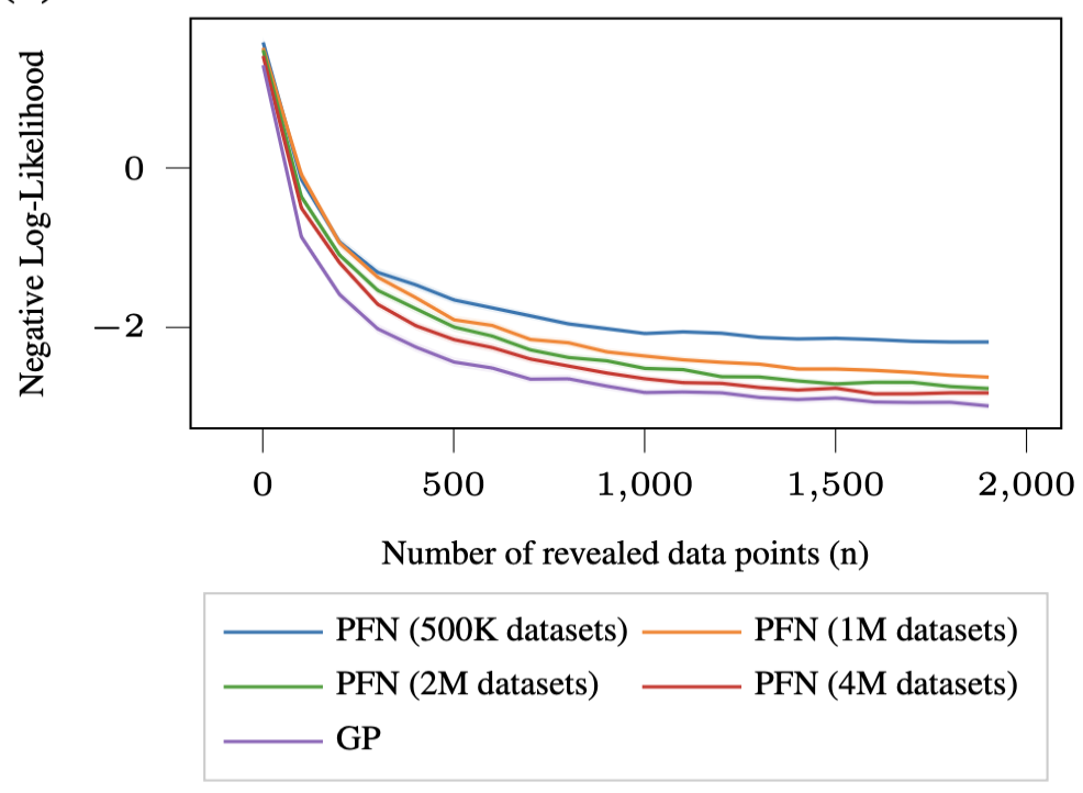
The result is that the PFN matches the GP posterior almost perfectly. The mean and confidence intervals are virtually indistinguishable from the ground truth, and the approximation gets better as you train on more synthetic datasets (from 500K to 4M).
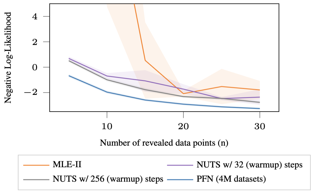
Gaussian Processes with Hyper-Priors
Now the GP hyperparameters are themselves random, drawn from a prior distribution. This makes the PPD intractable since you can no longer analytically integrate out the hyperparameters.
The baselines here are MLE-II (a special case of VI) and NUTS (the state-of-the-art MCMC sampler). The PFN not only achieves lower Prior-Data NLL than both baselines, it does so more than 200 times faster than MLE-II and between 1000 to 8000 times faster than NUTS.
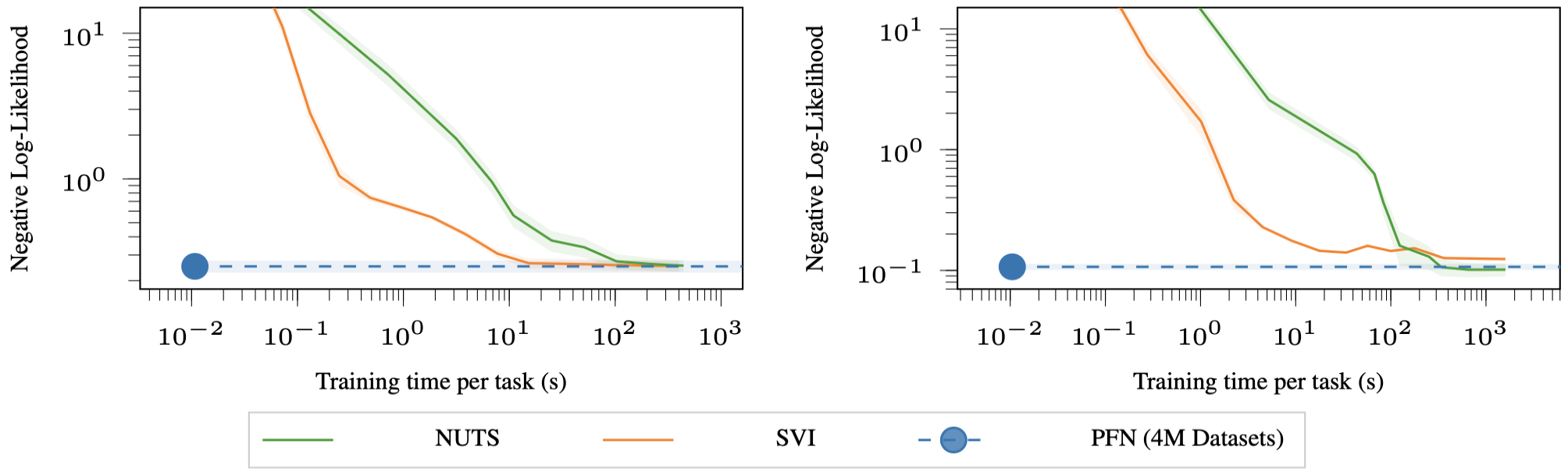
Bayesian Neural Networks
This is the hardest case and arguably the most important one. BNN posteriors are notorious for being complex, multimodal, and difficult to approximate. The baselines are Stochastic Variational Inference (SVI, specifically Bayes-by-Backprop) and NUTS.
To generate training data for the PFN, the authors sample random weights for a BNN, generate random inputs, and use the BNN’s outputs as labels. This gives them an infinite stream of synthetic datasets from the BNN prior.
The PFN achieves the same posterior approximation quality as SVI at 1000 times less compute, and the same quality as NUTS at 10,000 times less compute.
Why Is It So Fast? The Amortisation Perspective
The speed results above are striking, and they deserve a bit more explanation. The key concept is amortisation.
Think about what MCMC has to do every time you get a new dataset. It needs to run a Markov chain, wait for it to mix, collect samples, and then compute your prediction. All of that happens at inference time. For a Gaussian Process with hyper-priors and even a moderate dataset, this can take minutes.
PFNs pay all of this cost upfront during meta-training. When you train on millions of synthetic datasets from the prior, you are in effect pre-computing the answer to “what would Bayesian inference tell me, for any dataset that might come from this prior?” Once training is done, inference on a new dataset is just a lookup, implemented as a forward pass through the Transformer.
This is the same principle behind amortised variational inference in VAEs. A VAE trains an encoder network to predict the approximate posterior for any input image, instead of re-running an optimisation loop for each new image at test time. PFNs do something analogous but at the level of the PPD rather than the posterior of a single model.
The cost of amortisation is that you need to train the PFN once per prior, and that training can be expensive. But crucially, that trained PFN can then be reused for all future datasets that come from that prior, making the per-dataset inference cost essentially zero.
Limitations and Open Questions
PFNs are genuinely exciting, but it is worth being clear about where the current approach has limitations.
The prior must be sampleable. The only hard requirement for training a PFN is the ability to generate synthetic datasets from $p(\mathcal{D})$. For well-understood model classes like GPs and BNNs, this is straightforward. But for more exotic priors, it may not be obvious how to write a sampler. This is a softer constraint than what MCMC and VI require, but it is still a constraint.
Mismatch between prior and real data hurts. Like any Bayesian method, if the real data comes from a distribution that is very different from your prior, the posterior will be poorly calibrated. PFNs inherit this sensitivity. If your prior says “data is generated by a small BNN” but your real data is actually quite different, the PFN will not handle this gracefully.
Scaling to large datasets is hard. Transformers have an attention mechanism that is quadratic in the number of input tokens. If your training dataset has 10,000 examples, feeding all of them as tokens into a Transformer is expensive. The experiments in the paper focus on small to moderate dataset sizes, and scaling to larger settings is an open problem.
Approximation quality is bounded by model capacity. The PFN can only be as good as the Transformer model you train. If the true PPD is very complex and your model is not expressive enough, you will get a biased approximation. This is a different kind of bias than VI’s, but it is bias nonetheless.
Conclusion
For conclusion, let’s step back and appreciate how elegant this idea is:
Bayesian inference requires computing a posterior, which requires evaluating an intractable integral. MCMC and VI both attack this integral directly, at inference time, for every new dataset. PFNs instead ask: can we train a model that has already solved this problem for a whole family of priors, so that inference on any new dataset is trivially fast?
The answer, it turns out, is yes. And the key ingredients are a well-defined prior that you can sample from, a Transformer architecture that can handle set-valued variable-length inputs with permutation invariance, and a training objective that provably drives the model toward the true PPD.
The result is a method that can approximate Bayesian inference over Gaussian Processes and Bayesian Neural Networks orders of magnitude faster than MCMC or VI, with competitive or better accuracy. The code and trained models are available at the project GitHub, and the paper is here if you want to dig into the details.
What makes this particularly interesting is where it points. If you can specify a prior by writing a sampler, and then get fast, well-calibrated Bayesian inference for free at test time, the bottleneck for Bayesian deep learning shifts from “inference is too slow” to “can you write a good prior?” That is a much more tractable problem, and one where human domain knowledge can actually help.
Comments powered by Disqus.