TabPFN: A Single Forward Pass That Beats AutoML on Tabular Data

In the previous post, we looked at Prior-Data Fitted Networks (PFNs): a method that sidesteps the intractability of Bayesian inference by training a Transformer to directly approximate the posterior predictive distribution (PPD). The key idea was that if you can sample from a prior over datasets, you can train a model to do Bayesian inference in a single forward pass.

That post covered PFNs as a general framework. This post is about TabPFN, published at ICLR 2023, which takes the PFN idea and applies it concretely to one of the most common and stubborn problems in machine learning: classification on small tabular datasets. The result is a single pre-trained Transformer that can solve a new tabular classification problem in less than a second, with no hyperparameter tuning, and competitive with AutoML systems that are given an hour.

Let’s dig into how it works and why it is more interesting than it might first appear.

The Problem: Small Tabular Data Is Hard

Tabular data is everywhere. Clinical records, financial data, survey results, sensor logs. Despite being the most common data type in real-world machine learning, it is also one of the areas where deep learning has consistently underperformed compared to simpler methods. On small tabular datasets (say, a few hundred to a few thousand examples), Gradient Boosted Decision Trees like XGBoost and LightGBM almost always win.

Why? A few reasons. Neural networks tend to overfit on small datasets. They are sensitive to feature scaling and require careful hyperparameter tuning. And they make implicit assumptions about the data (such as smooth, low-frequency functions) that do not always hold for tabular data, where feature interactions can be irregular and non-monotone.

The standard solution is AutoML: run many models, tune their hyperparameters with cross-validation, and combine the best ones into an ensemble. This works well, but it is expensive. A system like Auto-sklearn or AutoGluon can take hours on a single dataset.

TabPFN asks a different question: what if we trained a single model once, offline, that already knows how to do all of this? What if fitting to a new dataset was just a forward pass?

The Core Idea: PFN Applied to Tabular Classification

TabPFN is a PFN. That means it is a Transformer trained offline on millions of synthetic datasets, to approximate the PPD in a single forward pass at test time.

The key ingredients, as with any PFN, are:

1. A prior over datasets that captures how real tabular data is generated
2. A training procedure that optimises the Transformer to approximate the PPD under that prior
3. An inference procedure that is just a forward pass

If you have read the previous post, steps 2 and 3 are the same as before. The thing that makes TabPFN interesting and technically novel is step 1: the design of the prior. Getting the prior right is what makes the model work well on real tabular data.

The Prior: Teaching the Model What Tabular Data Looks Like

A PFN can only be as good as its prior. If the prior generates datasets that look nothing like real tabular data, the model will not generalise to real problems. So the authors spent a lot of effort designing a prior that captures the structure of real tabular datasets.

The prior is a mixture of two components:

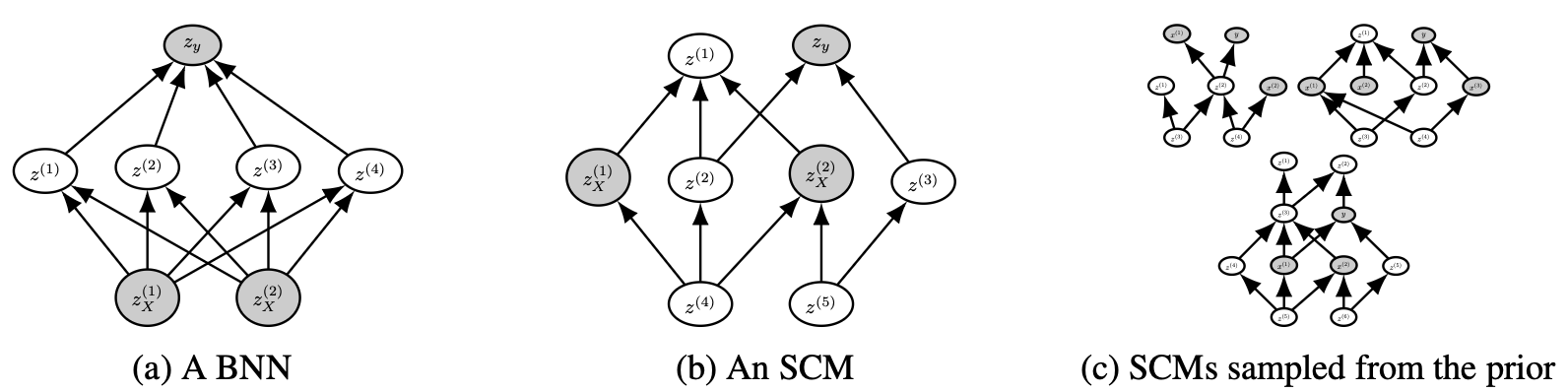
Structural Causal Models (SCMs)

The first component is based on Structural Causal Models. The intuition here is that tabular data often arises from causal processes. In a medical dataset, some features cause others. In a financial dataset, some variables are downstream effects of others. SCMs are a natural language for describing these kinds of relationships.

An SCM consists of a directed acyclic graph (DAG) where each node $z_i$ is computed from its parents:

where $f_i$ is a deterministic function and $\epsilon_i$ is a noise variable. To sample a dataset from this prior, the authors:

1. Sample a random DAG structure (similar to a sparse MLP)
2. Sample random weights for each edge
3. Sample a set of nodes to serve as input features and one node as the target
4. Generate $n$ samples by propagating noise through the graph

This gives a diverse family of datasets with correlated features, non-linear relationships, and causal structure, all of which are common in real tabular data.

Importantly, the prior has a simplicity bias: simpler graphs with fewer nodes and parameters are more likely. This is inspired by Occam’s Razor and reflects the fact that real-world data is often well-explained by relatively compact mechanisms, even if those mechanisms are non-linear.

Bayesian Neural Networks (BNNs)

The second component of the prior uses Bayesian Neural Networks, as in the original PFN paper. To sample a dataset, you sample random weights for a small neural network and use it to generate input-output pairs. This captures a complementary space of data-generating processes, with smoother and more global structure than the SCM prior.

During training, the TabPFN samples from the SCM prior and the BNN prior with equal probability, giving the model exposure to a wide variety of dataset types.

Additional Realism

Beyond the two main components, the prior includes several refinements to better match real tabular data:

Correlated features. In real tabular data, adjacent columns are often correlated. The SCM prior naturally produces this through its layered graph structure, and the authors exploit this by sampling feature nodes in adjacent blocks.

Irregular feature importance. In real datasets, some features matter much more than others. The prior handles this by sampling a separate weight multiplier for each input feature, amplifying differences in importance.

Categorical features. Tabular data often includes categorical variables. The prior generates these by binning continuous outputs into discrete categories, with a randomly sampled number of classes.

Varied noise distributions. Rather than assuming Gaussian noise everywhere, the prior samples separate noise distributions for each node in the graph.

All of this means the prior generates a genuinely diverse family of datasets that spans a large fraction of what you actually encounter in practice.

Training: One Time, Offline

With the prior defined, training is exactly the same as for any PFN. You repeatedly:

1. Sample a synthetic dataset from the prior
2. Hold out some examples as test points
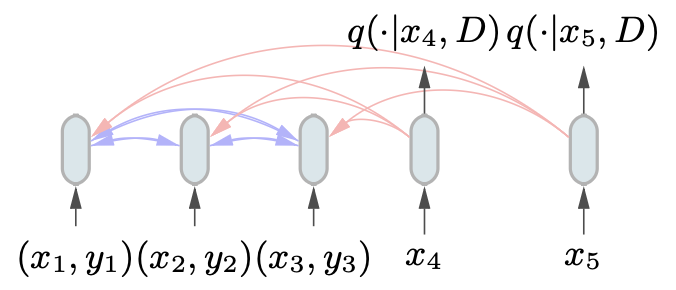
3. Feed the training examples and a test input $x$ into the Transformer
4. Predict the label of the held-out test point
5. Minimise the cross-entropy loss

As shown in the previous post, minimising this loss is equivalent to minimising the expected KL divergence between the model’s predicted distribution and the true PPD under the prior. So the model is being driven, directly and provably, toward Bayesian inference.

The TabPFN was trained for 18,000 steps with batches of 512 synthetic datasets, taking about 20 hours on 8 GPUs. That sounds like a lot, but it is a one-time cost. The resulting model is fixed and reused for every future dataset.

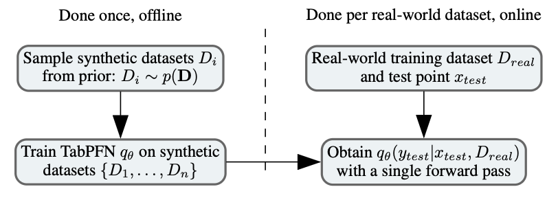
Inference: One Forward Pass

Once the TabPFN is trained, applying it to a new real-world dataset is straightforward. You just feed the training examples and a test input into the Transformer as a set, and read off the predicted class probabilities from the output. No fitting, no tuning, no optimisation. The whole process takes less than a second on a GPU.

This is the payoff of the amortisation idea from the previous post. All of the work of figuring out how to do Bayesian inference for tabular data was done during offline training. At test time, the model has already internalised everything it needs to know about how tabular datasets work, and it applies that knowledge instantly.

There is one important subtlety: the Transformer takes a set of training examples as input, not a sequence. This means the model is permutation invariant with respect to the training data, which is the right property: the order in which you list your training examples should not affect your predictions. This is achieved by removing positional encodings from the Transformer, exactly as in the original PFN paper.

Ensembling for Extra Performance

The authors also found that running 32 forward passes with different random permutations of the feature columns and class labels, and averaging the resulting predictions, gives a meaningful performance boost. This costs about 0.6 seconds on a GPU, still dramatically faster than any baseline.

What Does the Model Actually Learn?

One of the most interesting aspects of TabPFN is that it learns decision boundaries that reflect its prior. Because the prior prefers simple SCMs, the model tends to produce smooth, regular decision boundaries rather than the jagged, step-function-like boundaries you get from tree-based methods.

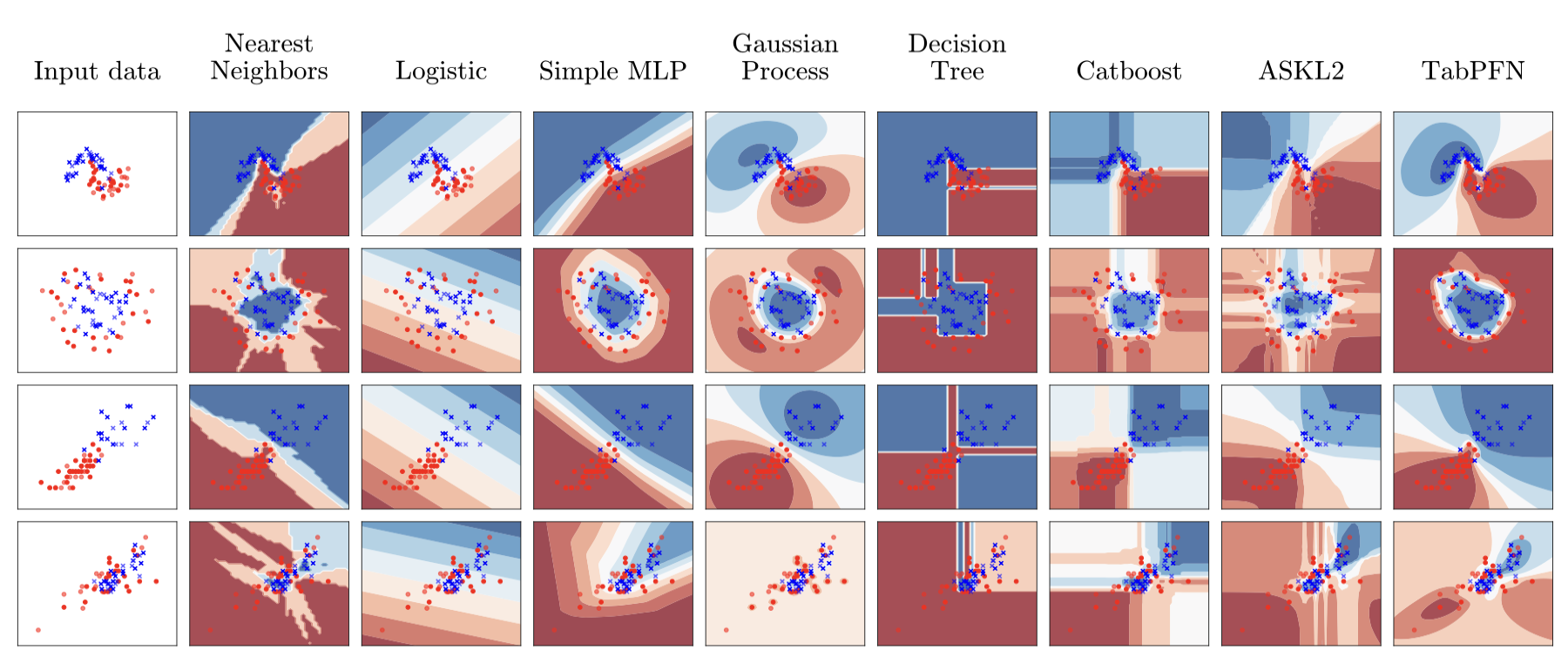
This is actually a feature, not a bug. Real-world classification problems are often better described by smooth boundaries than by highly irregular ones. The simplicity bias in the prior is acting as a form of regularisation, which is especially valuable when the training set is small.

The model also shows well-calibrated uncertainty. Because it is doing Bayesian inference under a sensible prior, it naturally produces high-confidence predictions near the training data and lower-confidence predictions far from it, similar to a Gaussian Process.

How Does It Perform?

The paper evaluates TabPFN on 18 purely numerical datasets from the OpenML-CC18 benchmark, with up to 1,000 training examples and up to 100 features.

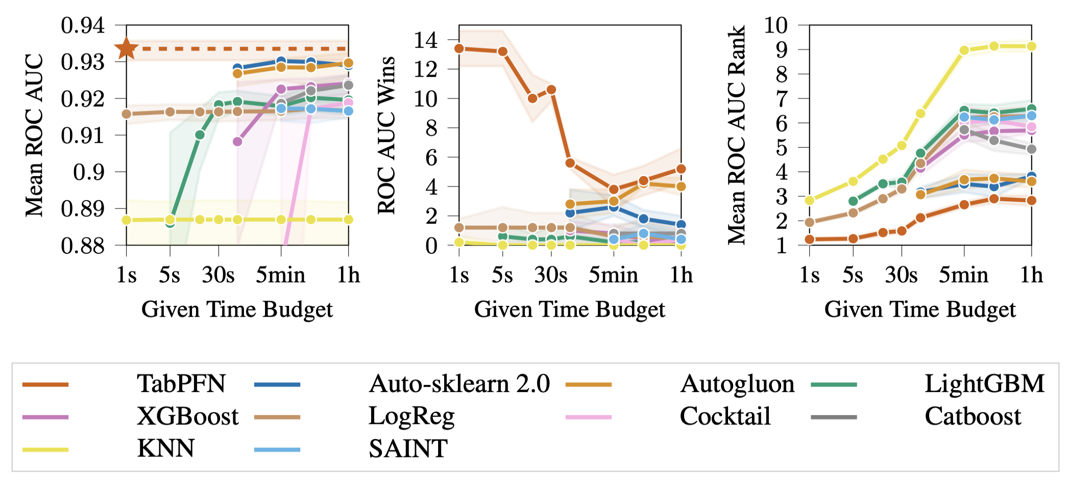
The headline result is striking. TabPFN on a GPU takes less than a second and matches the performance of the best AutoML systems (Auto-sklearn 2.0 and AutoGluon) given a full hour of compute. It clearly outperforms tuned XGBoost, LightGBM, and CatBoost in terms of ROC AUC, which have been the gold standard for tabular classification for years.

The speedup numbers are staggering. Compared to the best-performing AutoML system at the one-hour mark:

• TabPFN on CPU is 230 times faster
• TabPFN on GPU is 5,700 times faster

And the calibration is excellent too. The Expected Calibration Error (ECE) of TabPFN is 0.025, which is lower than every baseline including standard BNNs and XGBoost. This means when TabPFN says it is 80% confident, it is right about 80% of the time. That kind of calibration is very hard to get from standard methods without post-hoc calibration steps.

Why Does It Beat XGBoost?

This might seem surprising. XGBoost is a heavily engineered, highly optimised method with decades of community effort behind it. How does a single forward pass through a Transformer beat it?

The answer lies in what each method is doing. XGBoost fits a model to the specific dataset in front of it, with no prior knowledge about what kinds of patterns tend to appear in tabular data. It has to infer everything from the training examples alone. On a dataset with only 100 or 200 training examples, this is a hard problem, and you need careful cross-validation and hyperparameter tuning just to avoid overfitting.

TabPFN, on the other hand, has already seen millions of synthetic datasets during training. It has internalised a rich prior over what tabular data looks like, including correlations between features, causal structure, and the kinds of decision boundaries that tend to appear in practice. When it sees a new dataset, it is not starting from scratch. It is doing Bayesian inference under a well-calibrated prior, which means it naturally avoids overfitting on small datasets without any explicit regularisation.

In Bayesian terms, XGBoost is doing maximum likelihood estimation with a hand-crafted inductive bias. TabPFN is approximating full Bayesian inference under a data-driven prior. On small datasets, where there is a lot of uncertainty, Bayesian inference with a good prior reliably wins.

Limitations

TabPFN is impressive, but it is important to be clear about where it does not work well.

It only handles small datasets. The Transformer’s attention mechanism scales quadratically with the number of input tokens. TabPFN was trained with up to 1,024 training examples, and becomes expensive for larger datasets. For anything with more than a few thousand training examples, the performance advantage disappears and the cost becomes prohibitive.

It struggles with categorical features and missing values. The prior was designed primarily for numerical data, and the model performs significantly worse when categorical features or missing values are present. The authors acknowledge this and flag it as an area for future work.

It is sensitive to uninformative features. Adding a large number of irrelevant features hurts TabPFN more than it hurts tree-based methods, which are naturally robust to this through feature selection. This is related to the fact that TabPFN is somewhat rotationally invariant, which has the downside of making it harder to identify and ignore irrelevant features.

The prior has to fit the data. Like any Bayesian method, TabPFN’s advantage depends on the prior being a reasonable match for the data-generating process. If your dataset comes from a very unusual distribution that the SCM and BNN priors do not capture well, performance will degrade.

The Bigger Picture

TabPFN is a proof of concept for a broader idea: that the right way to do machine learning on small datasets is not to fit a model from scratch each time, but to pre-train a model that has already learned how data works, and then apply it instantly via Bayesian inference.

This shifts the bottleneck. Instead of “how do we build a better gradient boosting method?”, the question becomes “how do we design a better prior?” And that is a question where human domain knowledge can genuinely help. If you know something about the structure of your problem, such as that data tends to be generated by causal processes, or that simpler explanations are more likely, you can encode that directly into the prior and the PFN will automatically incorporate it into its predictions.

The paper’s code and pre-trained model are available at the project GitHub, and there is a scikit-learn-compatible interface, so you can use it in a few lines of Python. If you are working with small tabular datasets, it is worth trying before reaching for XGBoost.