Self-Supervision

Introduction

Self-supervised learning (SSL) is rapidly closing the gap with supervised methods. Very recently, Facebook AI Research (FAIR), one major player in broadening the horizon of self-supervised learning, introduced SEER. SEER is a 1.3B parameter self-supervised model pre-trained on 1B Instagram images that achieves 84.2% top-1 accuracy on ImageNet, comfortably surpassing all existing self-supervised models paper. Other researchers at FAIR trained Self-Supervised Vision Transformers (SSViT) and compared it to fully supervised ViTs and convnets, and found out that SSViTs learn more powerful representations [paper].

image source

In spite of all these recent break-throughs, the main idea behind self-supervision is not really new and it has been around for a while now, only under different names, mostly under unsupervised learning. However, there is a debate that we should stop seeing it as unsupervised, since it is not really “unsupervised” in the essence. In self-supervised learning, we are indeed supervising the model training, but with free and creative supervision signals instead of with human generated one. One very interesting and not much new example is Word2Vec paper, where we train a model to predict a word given its surrounding words. This paper came out at ICLR 2013 and the results were considered magical at that time. This paper showed that if you train such a model that tries to predict a word given its few previous and following words, the feature extractor extracts feature vectors with a lot of interesting linear relationships. For example, if we call the feature extractor f(), we can show that f(‘king’) - f(‘man’’) + f(‘woman’) = f(‘queen’). These early results showed self-supervision is fully capable of extracting semantic relationships.

It is true that supervised learning has been tremendously successful during the past decade, but we all know that we cannot label everything. If we want to move towards a system which forms generalized knowledge about the world and relies on its previously acquired background knowledge of how the world works, we need something bigger than supervised learning. We need to build systems which are capable of forming some sort of common sense about the world, just like human babies. As Yann Lecun elegantly put it, this common sense is the ‘dark matter of intelligence’, and he argues that this might be learned through self-supervision here.

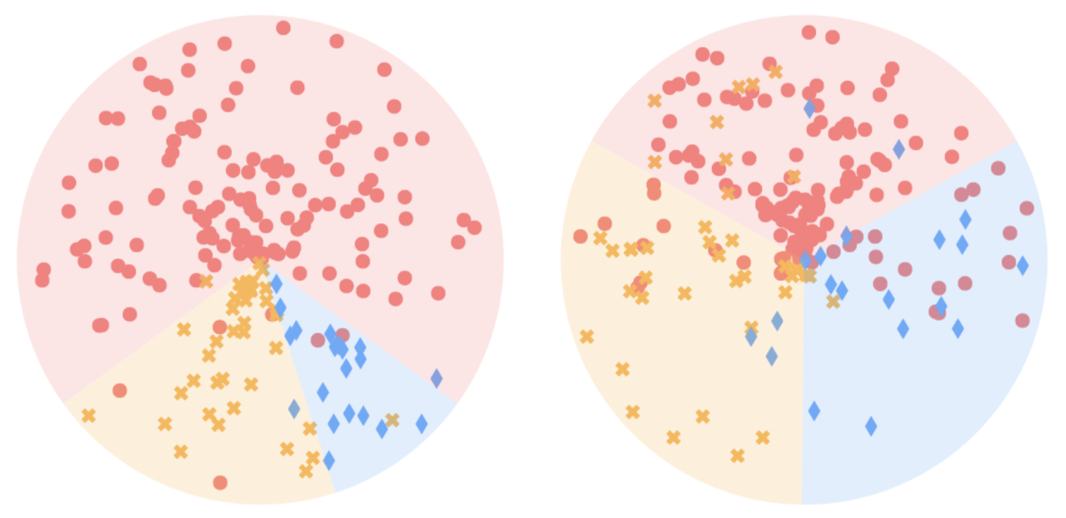
Well if you are not already curious and motivated enough to jump head first into the realm of self-supervised learning, let me introduce one recent paper which studied and compared the latent representation learning achieved from self-supervised learning and supervised learning in a very imbalanced setting, where there is not an equal number of each class in our training dataset. Authors conduct a series of studies on the performance of self-supervised contrastive learning and supervised learning methods over multiple balanced and imbalance datasets. They show that different from supervised methods with large performance drop, the self-supervised contrastive learning methods perform stably well even when the datasets are heavily imbalanced. Their further experiments also reveal that a representation model generating a balanced feature space can generalize better than that yielding an imbalanced one. Figure below visualizes the feature space learnt by supervised learning on the left hand side, and learned by self-supervised learning on the right hand side. The dataset has been unbalanced and as you can see the supervised model has inherited this unbalancedness and learned an unbalanced feature representation, which is not the case for the self-supervised model. Authors of this paper show that a model with balanced feature space generalizes much better than its counterpart with imbalance feature space.

Well, I think that’s enough for an intro. Here in this article I am going through some of the most recent and the most successful methods that use self-supervision to learn latent representations that are good enough for downstream tasks. I am planning to first go through different categories of self-supervised methods, explain briefly one or two methods in each category, and then explain the challenges in each category. At the end I am going to talk a little bit about self-supervision in Transfer Learning and more specifically, in Domain Adaptation, and introduce a recent method that uses self-supervision to better adapt to new domains.

Categories of SSL

Roughly speaking, current methods of SSL fall into one of these three categories: pretext task learning, contrastive learning, and non-contrastive learning

Pretext Task Learning

Pretext task learning tries to define creative pretext task problems that solving them teaches the model a good understanding of the semantics of our data. Next I am going to explain two of the most important works in pretext learning. The first one takes two patches of one image and tries to predict the relative location of the second patch to the first one. And I already spoiled the other method. It learns to solve a jigsaw puzzle. Let’s see how they achieve their goals!

Context Prediction

In this paper, authors train a CNN to classify the relative position between two image patches. One tile is kept in the middle of a 3x3 grid and the other tile can be placed in any of the other available 8 locations.

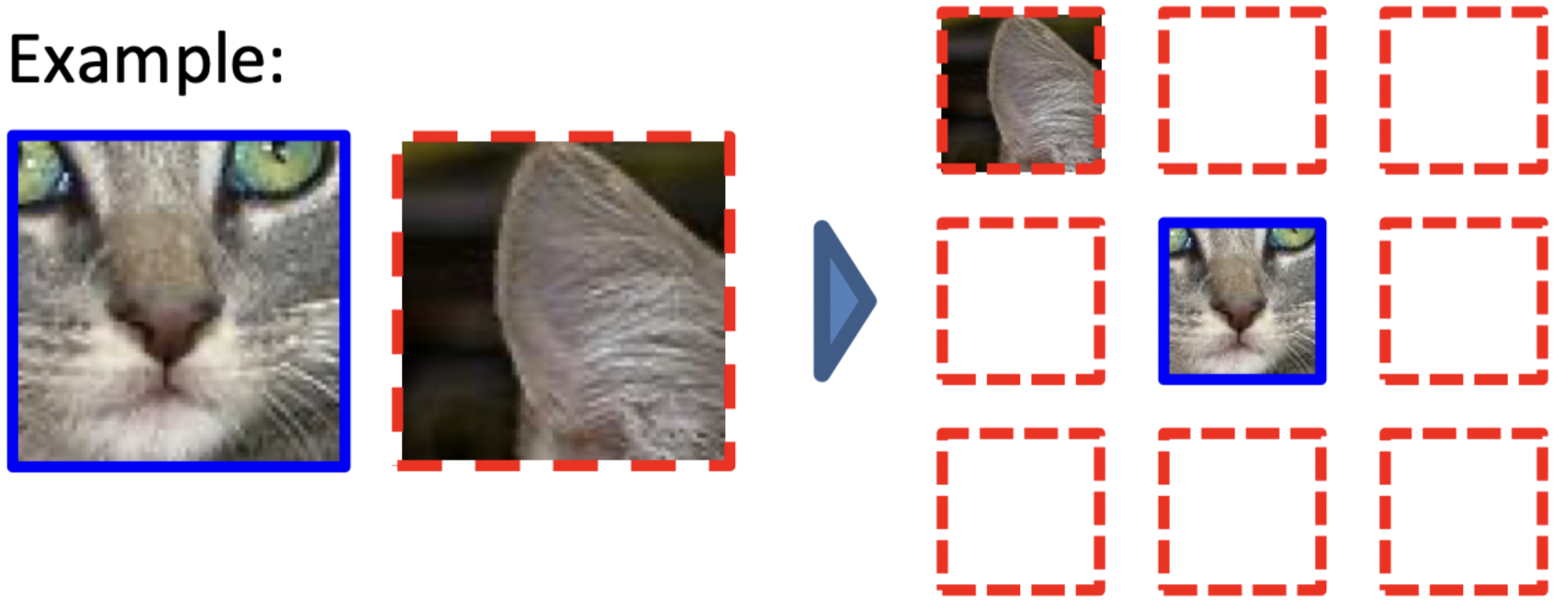
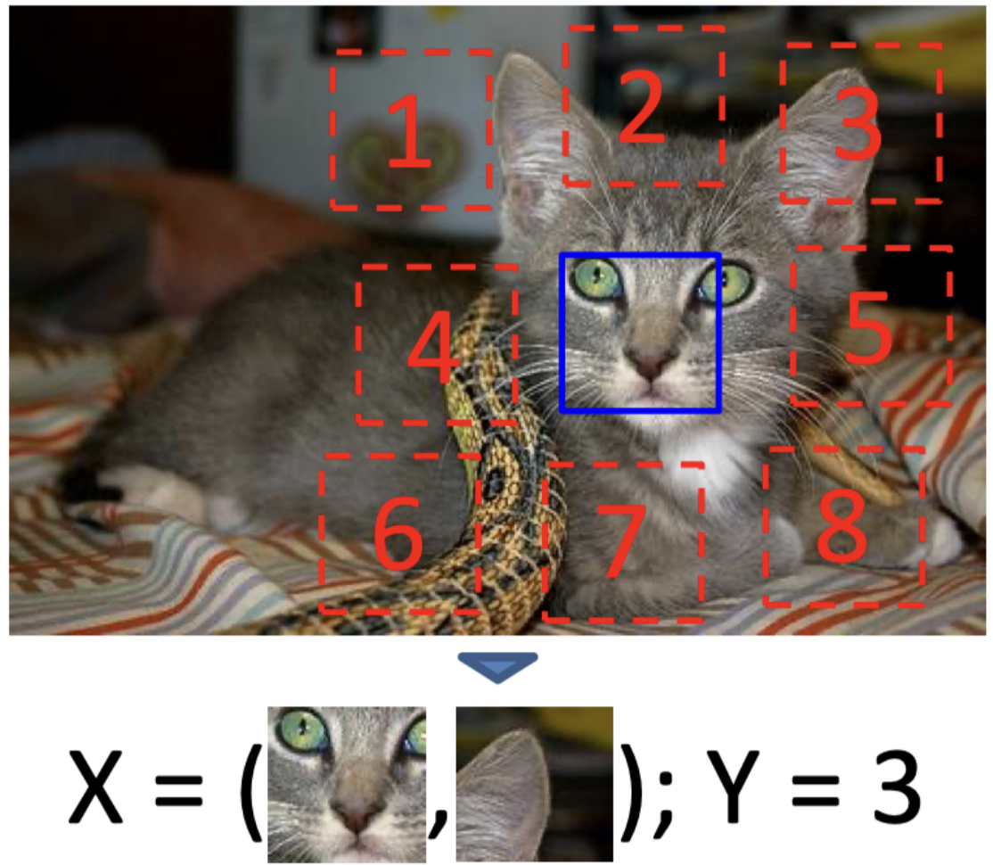
For example, given two above patches, the authors try to teach a model to predict 1, which is the relative position of the second patch to the first one. Or in the image below, we see that given those two images the model should predict Y=3

Authors achieve their goal by training two parallel CNN-based networks with shared weights. One network takes the first patch and the other one takes the second patch as input.

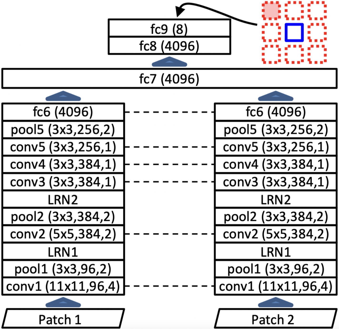
The architecture of the network is shown in the above picture. Each parallel network is following the AlexNet architecture as much as possible. The outputs of fc6 is then concatenated together to form the input for fc7. The output layer, fc9, has 8 neurons, each corresponding to one of 8 possible locations. Authors show that taking PASCAL challenge, their pretrained model beats AlexNet trained from scratch. However, this might not be the most fair comparison since the later one is not using any images outside of the PASCAL dataset, not just any labeled images.

Solving a jigsaw puzzle

The newer version of the previous paper is this paper, which takes this to another step and use jigsaw puzzle reassembly problem as their pretext task. Authors argue that solving Jigsaw puzzles can be used to teach a system that an object is made of parts and what these parts are.

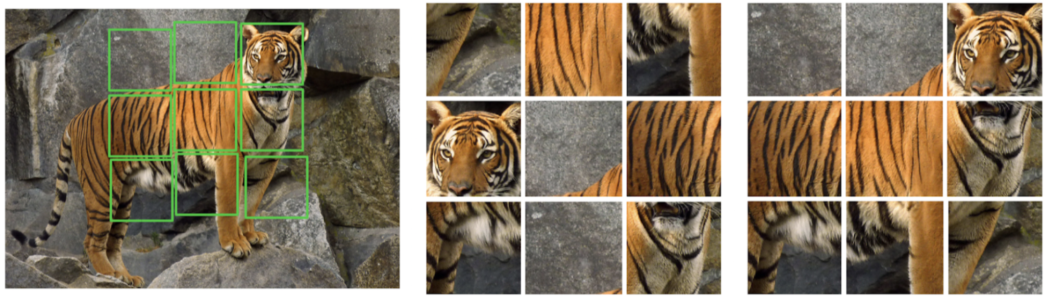
Above picture shows what they tend to do. Given this tiger photo, they want to randomly extract a 3x3 patch from it, randomize the tile, and train a network capable of predicting the correct location for each tile. This is achieved by 9 parallel CNN-based networks with shared weights.

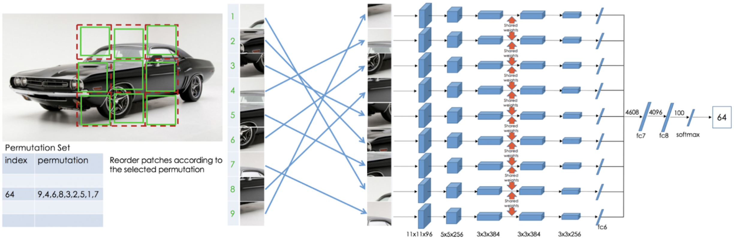
Authors define 64 different permutations for each puzzle, e.g. S=(8,4,1,9,7,3,6,5,2) and the network needs to predict which one of these 64 permutations it received as input. They show that their method beats the context prediction method with a high margin in the PASCAL challenge.

Contrastive Learning

The problem with pretext learning is that usually it is not easy to come up with a task that ends up in good feature extraction. There is another family of self-supervision methods –contrastive learning– which self-supervises using a different approach. Contrastive Learning tries to form positive samples for each input data x, and map x into a latent representations where x is close to its other positive mates. One big problem with this approach is called collapse, which happens when the model learns to map all inputs to an identical embedding to get the perfect result. To avoid that, we also need negative examples for each input x, which are mapped as far as possible to the feature vector of x.

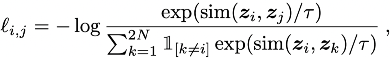
Above, you can see the a simple loss function for contrastive learning from this paper, where z_i is the latent representation for sample i, and sim() is a similarity function, e.g. cosine similarity. In this example, j is a positive pair for i, which is usually generated by corrupting sample i. In summary, we have N samples in each batch and we generate a positive pair for each of N samples so we have 2N samples in total. The goal is the latent representation of each sample, like z_i, to be as similar as possible to it’s positive examples, like z_j, and far from all other example in the batch and their corrupted version. So the rest of the current batch and their corrupted mate would play the role of negative samples.

As you might have already noticed, there is a lot that could go wrong here. The main questions are how do we want to choose positive and negative samples? For example, in the case of using corruption to generate positive samples, what is the best choice of corruption method? Or are the other samples in the batch good enough to be the negative samples? This is the choice of these negative samples that matters the most actually. An uncareful choice could end up in a collapse, or in inaccurate modeling of the loss function. For example, in the below demonstration, green dots, which are negative paris, need to be chosen carefully in order to get a good estimation of the loss function.

This a bigger issue in high-dimensional data, such as images, where there are many ways one image can be different from another. Finding a set of contrastive images that cover all the ways they can differ from a given image is a nearly impossible task. To paraphrase Leo Tolstoy’s Anna Karenina: “Happy families are all alike; every unhappy family is unhappy in its own way.” source This is why some researchers start look for novel non-contrastive methods.

Non-Contrastive Method

Non-contrastive methods are probably the hottest topic in self-supervised learning. Here I will introduce two of the most recent non-contrastive SSL methods. Once from Facebook AI Research and one from Deep Mind.

Barlow Twins

The first method, which is a work of Yann Lecun research group in FAIR, owes its name to neuroscientist H. Barlow’s redundancy-reduction principle applied to a pair of identical networks. The main idea is the cross-correlation matrix between the latent representations for two different distorted versions of one image should be as close to identical as possible. Cross-correlation matrix measures the relation of one signal –here latent representation– with another one; which here means it measures the relation between each latent feature of one distorted version, with all latent features of another distorted version of the same image. Below you can see a demonstration of Barlow Twins.

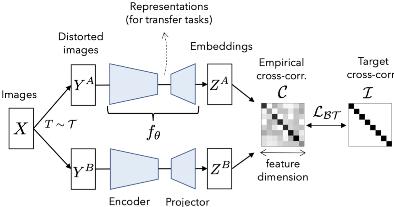
You might ask what is the point of having an identical cross-correlation matrix? Well, all diagonal elements of an identical matrix are one, which indicates the perfect correlation. Also all off-diagonal elements are zero, which means no correlation. In fact a diagonal cross-correlation matrix indicates that all latent variables of a same dimension have perfect correlation – similar representations for different distorted versions of a same image– and there is no redundancy between different components of latent representations.

BYOL

Bring your own liquor! Uh no I meant Bootstrap Your Own Latent representations. This is how researchers in Deep Mind decided to call their new non-contrastive method. Similar to every other method that I proposed in this article, this one also takes advantage of two parallel networks. But this time these two networks are not symmetric, nor identical.

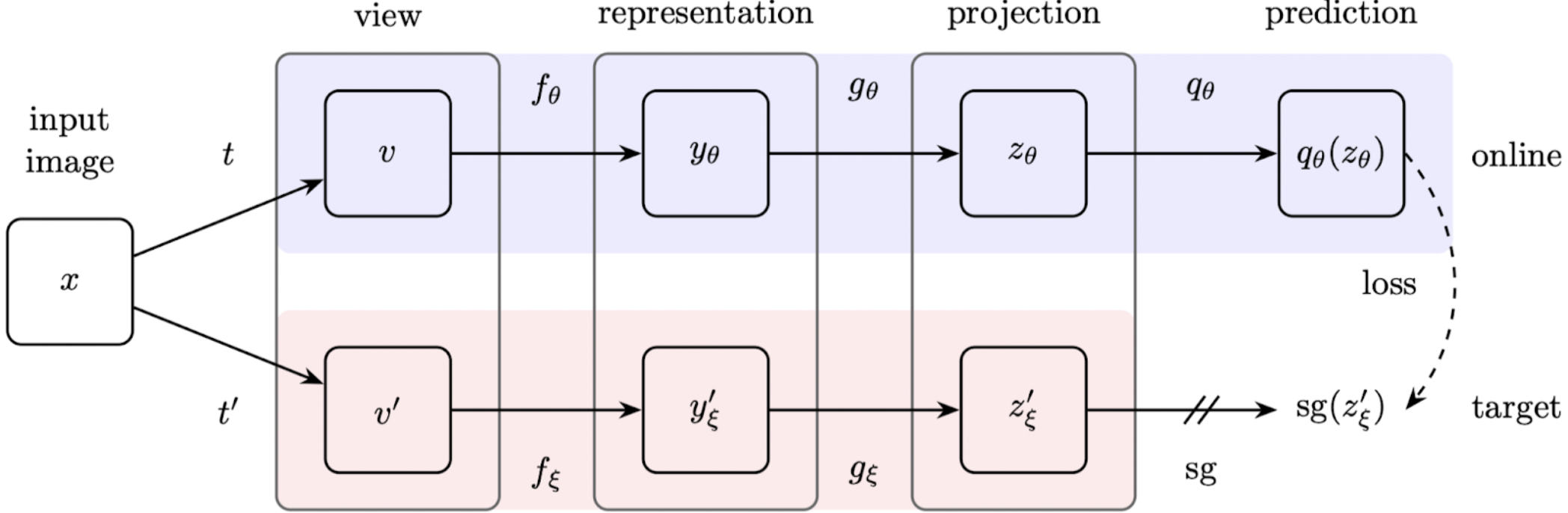
Both of these networks receive the same input image. However, they perform very different roles. Both of these networks have a representation component and a projection component which projects the input image into its latent representations. But the top network, which is called the online network, has one extra component compared to the bottom network, which is called the target network. This extra component, which is called the prediction component, receives the latent representation of the online network as its input and tries to predict the latent representation of the target network. The other difference between these two networks is how their parameters are updated. The online network is trained through stochastic gradient descent. However, the target network is trained using the slow moving average of the online network.

SSL in Domain Adaptation

One of the problems that SSL could be of some use in is Universal Domain Adaptation (UniDA). In UniDA we have a labeled source dataset from a domain, and an unlabled target dataset from another domain. Source and target dataset are sampled from different distribution and there is no constrain on their categories. This mean there might be classes in the source dataset that do not exist in the source dataset or vice versa.

UniDA naturally opens an opportunity to become creative and look for different forms of self-supervision that could be useful in either the distribution matching between the source and target domains or in the open class detection, where we want to detect target data that is from a target private only calss; a class that does not exists in our source dataset. This is what Saito et.al. do in the (DANCE)[https://arxiv.org/abs/2002.07953] method.

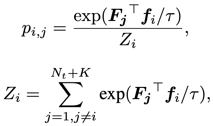
The idea behind the DANCE method is as follows: target data should either be clustered with source data so to be labelled as one of the known classes, or to form new clusters with other target data points. For this to happen, target points should either be pushed towards the current class prototypes or to get closer to the other data points. This can happen if we first define a similarity distributation for each data point, where p_ij shows how similar latent representation of point i is to F_j, where F_j is latent representation for either a class prototype or a target example. Then we can minimize the entropy of this distribution, so that we push our target latent representation towards F_j.

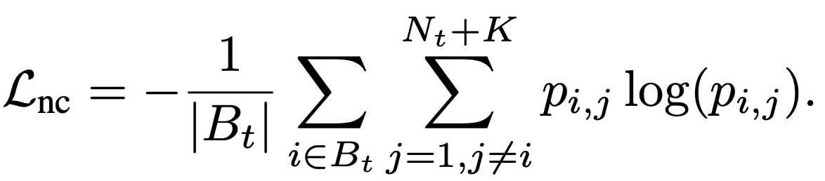
They call this term Neighbourhood Clustering.

The other term authors propose also uses entropy, but this time to align some of them with “known” source categories while keeping the “unknown” target samples far from the source. This loss term is called Entropy separation loss and we minimize it only if it’s distance from half of the max entorpy (rho) is larger than some threshold m. Please note that p is the classification output for a target sample.